We all know about cartographers and maps on paper or on screen. But “mapping” is a term used also by weathermen, artists, engineers, mathematicians, and scientists; “mapping” has a much broader definition when used for different maps.
Mathematical Mapping
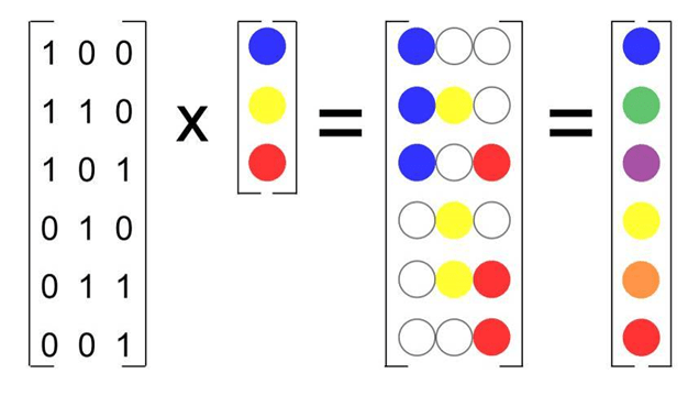
Mapping is a concept of matrix algebra, workhorse of modern computing. It is used to mathematically map one set of units (colors, coordinates, data points) into a new set of units. I love the example in the image below of mathematical mapping, because one set of colors – instead of numbers – is mapped into another set of colors using matrix algebra. Colors help make the concept intuitively understood.
The 6 x 3 matrix – ones and zeros – is a transformation matrix, which will be multiplied times the vector set of primary colors (blue, yellow, red). The middle matrix (after the 1st = sign) shows the result of multiplication.
After multiplication, each unit in each row of colors in the middle matrix are then added together to give the final, resulting color in rows of the final matrix (after the 2nd = sign). For instance, the 2nd row of the middle matrix is (blue, yellow, blank). Blue + yellow + blank = green, shown in the 2nd row of the final matrix.
The transformation matrix (one’s and zero’s) maps (transforms) the set of 3 primary colors blue, yellow, and red into a set of 6 primary and secondary colors blue, green, purple, yellow, orange, and red.
In my old mathematics professor’s non-intuitive language, the transformation matrix of ones and zeroes maps between spatial dimensions: “a primary color 3-space is mapped to a primary-plus-secondary color 6-space”.
Durer’s Ray Tracing Maps
Albrecht Durer (1471-1528) used mapping in his artwork. Of course, he did not have a computer and had never heard of transformation matrices. By using a physical apparatus, he invented ray tracing which enabled him to incorporate accurate perspective and proportion in his artwork.
Several of Durer’s own drawings show actual applications of his ray tracing tools and techniques, including one (below left) with a frame placed at a constant location between a mandolin and a viewer’s stationary eye (point A).

With point A’s position kept constant, straight lines (rays) of string from A to points on the instrument intercepted the frame’s plane at different points, each of which were measured relative to the frame (above, right) in x and y directions. Plotted points – C1, C2, C3 – became preliminary geometry work points for his final 2D sketch of the mandolin (above, right), viewed from point A. By using this apparatus and method, the final 2D sketch was appropriately “distorted” for perspective and proportion using ray tracing.
In mathematical terms Durer’s ray tracing apparatus and tools mapped (transformed) 3D geometry of the mandolin onto a 2D plane of artwork, where the viewer’s eye was positioned at point A. He understood reflected light travels in straight rays which converge on a viewer’s eye, and a viewer then sees accurate perspective and proportion in the mandolin and its surroundings.
Today, 500 years after Durer, ray tracing of reflected light and source lighting is used in more complex, mathematical forms in computer animation technology to accurately depict proportion, perspective, and lighting to heighten realism in animations.
Transferring Data to Weather Maps
Before television, radar, and weather satellites, 1870 weather maps were based on weather data information sent to central location by telegraph from various regional locations. They were primitive. But before telegraphs and telephones, useful weather maps did not even exist.
In the later 1800s and early 1900s, telegraph (and then telephone) made it possible to collect weather data every few hours simultaneously from weather stations over a large region. A weather map for a given date and time was made from the simultaneously collected data.
Data – barometric pressure, temperature, or wind speed – were collected using instruments, since all the information were invisible quantities.
Eastern U.S. maps (below), dated 1872, show barometric pressure lines and wind data collected from weather stations in eastern states at specified times. Subsequent maps made every few hours were used to track a fast-moving storm as it headed north from Florida. Date and time for plots are (clockwise from upper left): March 1, 11:35 pm, March 2, 7:35 am, March 2, 4:35 pm, and March 2, 11:35 pm.
Each map was made using simultaneously collected data from far-flung weather station observers across the southeastern US. Weather data reports were sent to headquarters by telegraph. Collected weather data was then transferred by hand (mapped) onto a background map of the southeast US, creating a series of sequential paper weather maps. Weather mapping was a team event, requiring many observers reporting via telegraph over a large region of the U.S. Each map took a few hours.

Next time I see a radar weather map of a storm moving effortlessly across my monitor screen, I’ll remember these primitive maps produced using the latest telegraph technology and hundreds of observers.
Kepler’s Mapping of Mars’ Orbit
To understand the brilliance of Kepler (born 1571) in imagining and then mapping Mars’ orbit, one first must visualize patterns Kepler saw in the night sky. Patterns of Mars’ movements seen in the sky are so different than patterns Kepler finally imagined and mapped as Mars’ orbit.
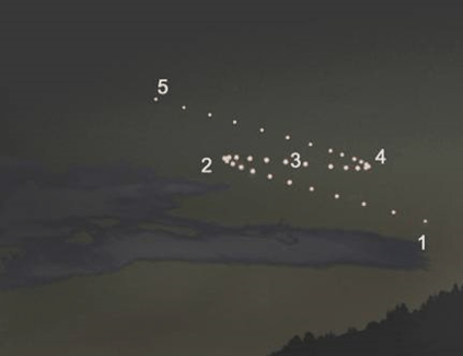
At first, it appears Mars orbits Earth. But several plots of Mars’ position over time will show Mars does not move smoothly across the sky. At times Mars moves forward, then backwards for a bit before moving forward again – in so-called “retrograde” motion, as seen in the night sky image #1 (above). Mars’ position moves from 1 to 2 then 3, 4, 5.
Earlier observers – Plato, Aristotle, Ptolemy – also noticed retrograde Mars motion. But they imagined an incorrect solar system model – one where planets orbited Earth. Any theories based on this earth-centered model were doomed to be incorrect.
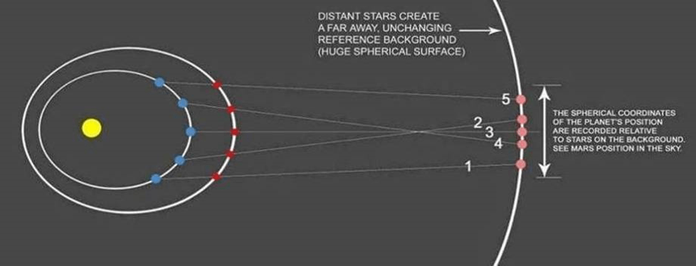
Because Kepler had imagination to correctly interpret this weird retrograde motion, he finally made a correct map of Mars’ orbit. Mars’ orbit lies in a flat, plane. To see Mars’ orbital plane, one would need to be far above the solar system, looking straight down on Mars’ flat orbital plane. The planetary orbital plane image #2 (below) shows dark red dots indicating Mars’ orbit around a yellow sun, while Earth’s orbit has blue dots.
Because we view Mars’ position from Earth, we don’t see the true orbital plane as in this view of the orbits. We see Mars’ orbital plane from Earth’s orbital plane. And for practical purposes, Mars’ orbit and Earth’s orbit lie in the same plane.
Thanks to Kepler, we now understand Mars’ retrograde motion to be caused by relative positions of Earth’s solar orbit and Mars’ solar orbit. Mars is further from the sun than Earth, and we see Mars against a far distant background of stars that appears motionless. At first, Mars tends to appear to move faster than Earth against the starry background (points 1 to 2 in both images #1 and #2). However, when Earth and Mars move parallel to each other, Mars appears to fall behind. Earth appears to move faster relative to Mars (points 2 to 3 to 4 in both images). Earth’s smaller orbit makes it turn sooner than Mars does so Earth appears to slow down. This allows Mars to appear to move faster once again (point 5 in both images). Kepler interpreted this motion accurately.
Kepler had access to Tycho Brahe’s extensive and accurate observational measurements of Mars’ position. Wanting to know the geometrical shape of Mars’ planar orbit, he transformed (mapped) measurements observed from Earth to positions along Mars’ orbital plane. He assumed different mathematical orbital shapes – circular, oval, elliptical – and performed calculations which predicted Mars’ location in the sky for each assumed shape. These calculations were tedious and time-consuming, given mathematical knowledge at the time.
Eventually Kepler created a mathematical map of Mars’ orbit using an ellipse with the sun at one focus, which predicted Mars’ observed position accurately. Kepler’s First Law states a planets’ orbit is an ellipse with the sun at one elliptical focus. An elliptical planetary orbit is shown in planetary elliptical orbit image #3 (below) together with a modern mathematical formulation.
Kepler displayed some amazing and imaginative geometry skills.

Durer’s Human Face Maps
Durer used mapping in another form. He mapped sketches of faces over grid lines in the image below, such as a normal profile below (A) to accurately define geometry of faces. These graphical maps enabled him to classify individual facial differences among facial constructions using intuitive transformational mapping. Durer studied the geometrical patterns of faces for his artwork.
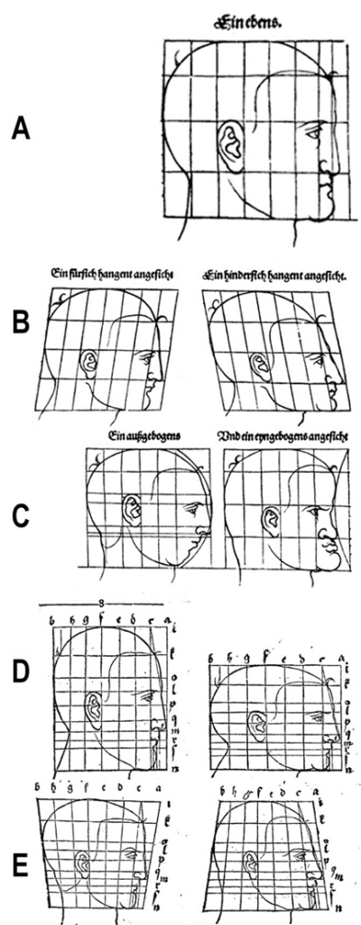
He transformed grids over his normal profile (A) to create new faces.
With a rectilinear grid over normal profile (A), Durer skewed grids right or left, transforming the profile into new facial profiles (B).
He added convex or concave grids, moved grids, and transformed profiles to the curved grids, creating new characters.
As he explored new ways of transforming grid lines, he added grid lines and made taller and shorter profiles (D) by changing the distance between grid lines.
In (E), he linearly adjusted dimensions between grid lines from top to bottom to create new faces.
These methods of experimenting with grid lines gave him many new facial profiles for his art.
Mapping Constellations
According to legend, Orion was son to Poseidon and Euryale, daughter of Minos, King of Crete. In Crete, Orion, a mighty hunter, hunted with goddess Artemis and boastfully threatened to kill all of Earth’s beasts. Apollo, sister to Artemis, objected and sent a giant scorpion to kill Orion.
After Orion’s death, Zeus placed Orion among stars as a constellation. Zeus also added the constellation Scorpio, the scorpion, as tribute to Orion. Scorpio, however, is placed so it is not visible concurrently with Orion. Orion is an easily recognizable constellation with three bright stars in his belt (below, left). Stargazers in India, Persia, Europe, and China all had their own images of Orion (below, right 6 images), created by artists who used imaginations and cultural heritages to connect the star dots to form a unique image.
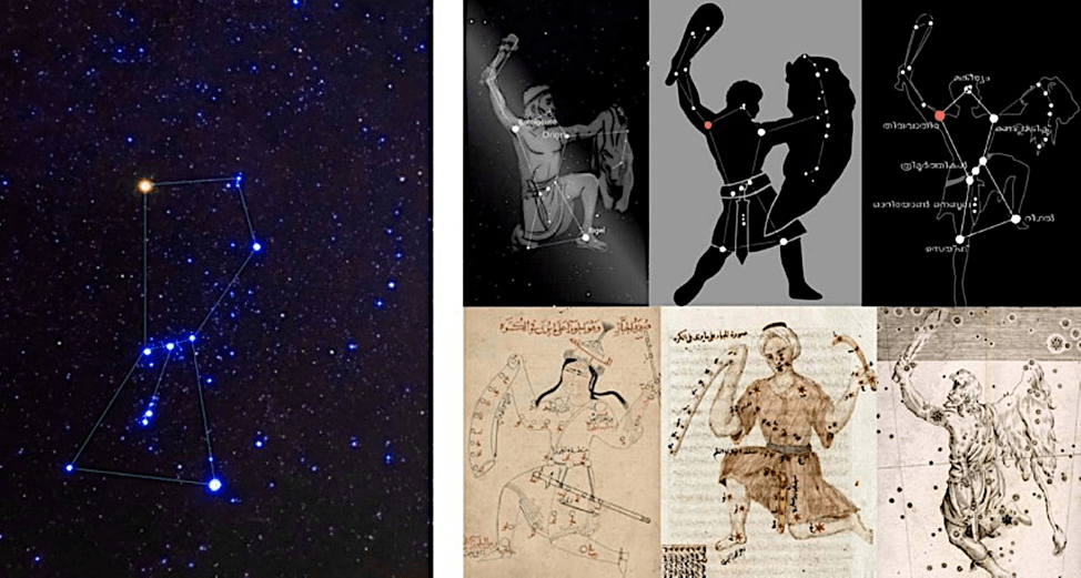
The constellation Orion, like all constellations, is an imaginary pattern of stars. Yet, all constellations are important aids to memorization – mnemonics – for us to use in observing or mapping the night skyscape. Constellations orient us towards north and south, mark the changing seasons, and serve as markers for navigation, useful to mariners, hikers, and pilots.
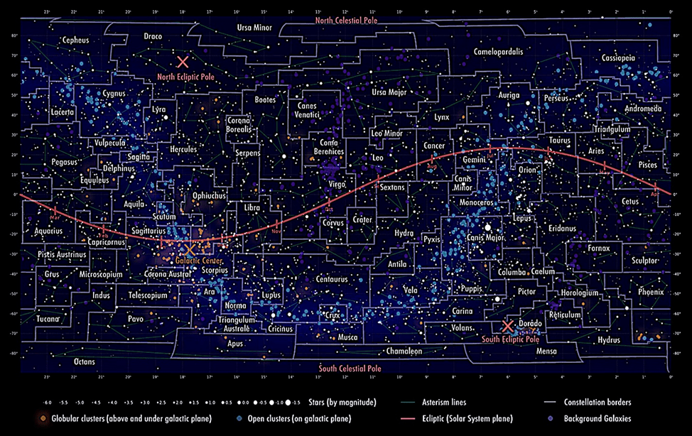
Constellations are still important mnemonic markers today. Each constellation recognized by the International Astronomical Union (IAU), founded 1919, now has its own boundary, established by the IAU and marked in spherical coordinates. Through the IAU, constellations are accurately mapped (see below). Patterns of constellations and their boundaries are imaginary, yet constellation boundaries established on IAU maps are real and serve real navigation and scientific purposes in locating objects in the sky. Constellation boundaries have become an international, measurable geometrical framework with coordinates and arc lengths that are as real as state boundaries.
Simple, Familiar Roadmaps

Examples above for various forms of mapping are not so different than the simple road map (left above). A road map is also a transformation of data from one space (the real 3D world) shows roads, rivers, lakes, airports, cities, and other transportation features. But it is not a scale model nor an exact replica; instead, it uses symbols, lines, shapes, and colors to represent real features. If we understand the map symbols, we can use the map for driving.
A cartographer uses symbols to make road maps by transferring, or mapping, real locations of roads, rivers, and cities from their actual positions to their corresponding locations on flat paper or flat screen. Corresponding maps are drawn as scaled versions of reality, transferring information via coordinates and a grid system.
This is a simple form of mapping, defined as a “an operation that associates each element of a given set (real 3D objects) with one or more elements of a second set (the map in 2D).” Roadmaps are mathematical, geometrical, and symbolic.
Topographic maps (right above) are a bit more complex than road maps. Topo maps have 2D information common with road maps – roads, trails, rivers, cities. But topographical maps also transfer (or map) another piece of information at each point – elevation above sea level – to the map by using added contour lines. Curving contour lines connect coordinate points which have the same elevation on a topographic map’s flat surface. It’s a clever way of showing a 3rd dimension – elevation – on a 2-D paper or screen surface.

Leave a comment